
Small Signal Stability in Power Systems: Analysis, Oscillatory Modes and Renewable Integration
Small signal stability is a power system’s ability to maintain synchronism when it experiences small disturbances such as normal variations in load and generation. Linearized models are used to determine whether oscillations decay, persist, or grow around a selected operating point.
Introduction
Power systems are moving from centralized networks dominated by synchronous machines towards increasingly distributed, inverter-based architectures. This transition is changing the way dynamic stability is assessed. As renewable penetration increases, system inertia can decline, grid strength can weaken, and oscillatory behaviour can become more sensitive. Small signal stability (SSS) has therefore become increasingly important in understanding how a power system responds to the small disturbances that occur during normal operation.
Small signal stability is assessed using linearized state-space models and eigenvalue analysis to identify oscillatory modes, damping ratios (ζ), and frequencies (ω). When damping torque is insufficient, electromechanical oscillations may persist or grow after minor disturbances. The purpose of the analysis is to identify these modes, understand the components that participate in them, and determine whether the system has adequate damping at the operating point being studied. Depending on the applicable grid-code or system-operator requirements, SSS assessment may also form part of a broader grid-connection or compliance study.
Renewable integration adds another layer to small signal stability assessment. Solar and wind generation increasingly rely on power electronic converters rather than conventional synchronous machines that inherently contribute inertia and damping. Grid-following and grid-forming converters introduce fast control loops, including phase-locked loops (PLLs) and voltage and current controllers, which can interact with network dynamics. These interactions can create control-driven or sub-synchronous oscillatory behaviour that is not captured by classical synchronous-machine-only analysis, making detailed modal assessment more important in power-electronics-intensive grids.
Fundamentals of Small Signal Stability
Definition and Physical Interpretation
The term "small" refers to disturbances that are limited enough for the system response to be represented accurately by a linearized model. In practice, these include the continuous variations in load and generation that occur during normal operation, as well as minor switching events and small mismatches introduced by automatic generation control actions.
The physical behaviour of small signal stability can be understood through the balance between synchronizing torque (Ts) and damping torque (Td) acting on each rotating machine. If a synchronous generator rotor moves slightly away from its equilibrium position, synchronizing torque acts to restore the rotor angle, while damping torque opposes the speed deviation and dissipates oscillatory energy. A stable response therefore requires sufficient synchronizing torque to provide the restoring force and sufficient damping torque to allow the oscillation to decay.
When synchronizing torque is adequate but damping torque is insufficient, oscillations can remain sustained or grow. This is the central concern in small signal stability analysis. Eigenvalue-based methods are used to reveal the modal structure of the system and determine which modes require closer attention.
Linearization and State-Space Representation
Small signal stability analysis begins with the differential equations that describe the system and the relationship between its input, state, and output variables. These equations are then linearized around a selected operating point and expressed in state-space form:
ẋ = Ax + Bu
Where,
x= vector of state variable deviations from equilibrium,
A= state matrix capturing the linearized system dynamics,
B= input matrix,
u= small changes in inputs.
For stability analysis, the input change is typically set to zero, reducing the system to the reduced form:
ẋ = Ax
The eigenvalues of the state matrix (A) completely characterize the small signal dynamic behaviour. Each eigenvalue (λ) satisfies the characteristic equation:
det(A − λI) = 0
For an n × n state matrix, n eigenvalues are obtained. They may be real or occur as complex-conjugate pairs.
For a second-order system, the characteristic equation can be represented in terms of its eigenvalues as:
λ² + 2ζωₙ + ωₙ² = 0
Hence, solving the above equation for eigenvalues, we have;
λ = −ζωₙ ± jωₙ√(̅1̅−̅ζ̅²̅)̅ = σ ± jω
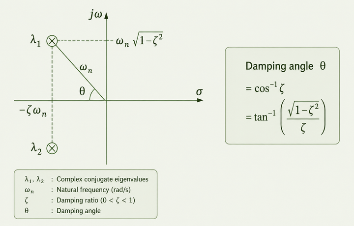
Figure 1: Location of eigenvalues in complex plane wrt ζ and ωn
The damping ratio (ζ) governs how quickly an oscillatory response decays, while angular frequency (ω) determines the timescale of the oscillation.
Swing Equation
For a single-machine-infinite-bus (SMIB) system, the swing equation describes the balance between mechanical torque (Tm) and electromagnetic torque (Te):
Md²δdt² + Ddδdt = Pₘ − Pₑ = Pₐ
Here,
M= inertia constant (proportional to the kinetic energy stored in the rotating mass),
D= mechanical damping coefficient,
δ= rotor angle referenced to a synchronously rotating frame,
Pm= mechanical power input from the prime mover,
Pe= electrical power output, and
Pa= accelerating power.
A positive accelerating-power imbalance causes the rotor to accelerate, while a negative imbalance causes it to decelerate.
Around a steady-state operating point δ0, Pm and Pe0, small changes in mechanical power ΔPm and electrical power ΔPe lead to the linearized swing equation:
Md²Δδdt² + DdΔδdt = ΔPₘ − dPₑdδ|δ₀ · Δδ
Using the selected state variables, the system can be written as a second-order state-space model. Its eigenvalues indicate whether the resulting angular oscillations will decay, persist, or grow.
Eigenvalues, Damping, and Oscillation Frequency
A complex eigenvalue corresponds to an oscillatory mode. Its imaginary component determines the oscillation frequency, while its real component determines whether the oscillation is damped or grows with time. The damping ratio ζ expresses the rate of oscillation decay relative to the undamped natural frequency:
ζ = −σ√(̅σ̅²̅ ̅+̅ ̅ω̅²̅)̅
When,
σ < 0 (i.e. ζ > 0): oscillations decay exponentially, and the mode is stable,
σ > 0 (i.e. ζ < 0): oscillations grow, indicating instability,
Real part of λ = 0 (ζ = 0): oscillations remain at constant amplitude, representing a marginally stable condition.
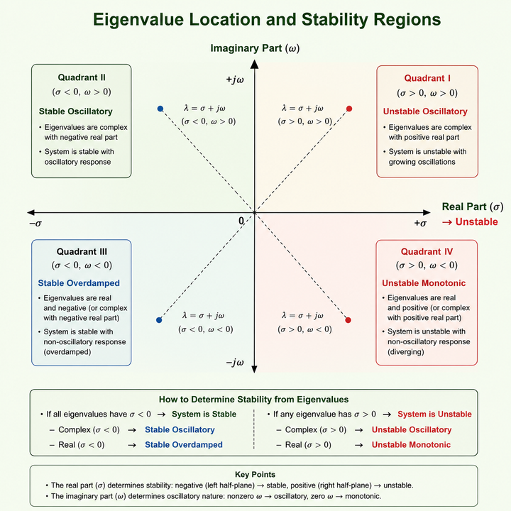
Figure 2: Interpretation of system stability based on Eigenvalue
Practical acceptance criteria are set by the applicable grid code, system operator, or project-specific requirement. Damping ratios in the 3–5% range are commonly used as screening benchmarks, but the governing criterion should be confirmed for the specific study. Modes below the applicable threshold can indicate inadequate damping and may lead to sustained oscillations under certain operating conditions.
Participation Factors
Eigenvalues show whether a mode is stable and how quickly it decays or grows, but they do not by themselves show which states or components are most responsible. Participation factors provide that link by quantifying how strongly each state variable contributes to each mode. For an eigenvalue (λi), with associated right eigenvector (Φi) and left eigenvector (Ψi), the participation factor of state variable k in mode i is:
pₖᵢ = φₖᵢψₖᵢ
Participation factors are dimensionless and normalized for each mode. They help identify the states and machines most involved in a critical oscillation and therefore support controller placement and tuning. For example, a power system stabilizer applied to a generator with high participation in a critical mode is likely to influence that mode more directly than one installed on a machine with negligible participation.
Small Signal Stability vs Transient Stability
Small signal stability concerns a system’s response to small, continuous disturbances and is assessed using linearized, eigenvalue-based methods. Transient stability concerns the response to large disturbances, such as faults or a sudden loss of generation, and requires nonlinear time-domain simulation because the system can move far from its original operating point.
| Aspect | Small signal stability | Transient stability |
|---|---|---|
| Disturbance | Small, continuous or minor disturbances | Large disturbances such as faults or sudden generation loss |
| Analysis approach | Linearized state-space and eigenvalue-based analysis | Nonlinear time-domain simulation |
Classification of Oscillatory Modes
In large interconnected power systems, oscillatory behaviour is typically grouped into four broad mode types: local, inter-area, control, and torsional. Each differs in its typical frequency range, dominant cause, and potential system impact.
| Oscillatory Modes | Typical Frequency Band | Typical Damping | Cause | Impact |
|---|---|---|---|---|
| Local | 0.8-2.0 Hz | Moderate to high | Generator swing vs. local load/network | Local overheating, relay mal-operation |
| Interarea | 0.1-0.8 Hz | Low | Large regions swinging against each other, high power transfer | Widearea power swings, tieline stress |
| Control | 0.5-5.0 Hz | Variable | Exciters, governors, PSS, HVDC, FACTS | Interaction with other modes, tuning issues (depends on controller location) |
| Torsional | 10-50 Hz | Very low (when excited) | Series compensation, converter controls | Sub-synchronous resonance phenomena, Torsional fatigue in turbine-generator shaft |
Small Signal Stability Modelling
A credible small signal stability study depends on appropriate representation of plant, control systems, and network dynamics. The component models need to capture the states and control loops that materially influence system eigenmodes and damping.
| Topic | Typical model elements / states | Key control loops or devices | Effects on small-signal stability | Tuning/modelling |
|---|---|---|---|---|
| Synchronous machine (detailed / two-axis) | Direct & quadrature axis flux linkages, field winding, damper windings, magnetic saturation, rotor angle & speed | AVR, PSS, governor (external) included in full model | Accurate representation of local and inter-area modes, interaction with exciter/governor | Using Park's transform |
| Excitation system (AVR) | AVR states; voltage setpoint, regulator integrators/filters | High-gain AVR, voltage measurement | Can improve transient response but excessive gain may reduce damping and introduce oscillations | Model AVR limits, delays, and saturation; include PSS when present |
| Governor / prime mover | Speed governor states, droop, valve/turbine dynamics, mechanical power | Speed sensing, droop control, valve actuator | Affects frequency damping and slow modes; interacts with system frequency during large disturbances | Include droop and valve dynamics; model for low-inertia grids |
| Power System Stabilizer (PSS) | Washout filter state, lead-lag compensators, PSS gain | Supplementary input to AVR (from speed or electrical power) | Adds positive damping to rotor oscillations when tuned correctly | Tune using eigenvalue analysis and participation factors; washout removes steady bias |
| FACTS devices (SVC, STATCOM, TCSC, UPFC) | Device internal control states, series/reactive compensation states, converters/thyristor dynamics | Fast power-electronic control loops, voltage/reactive/series control | Can provide strong damping when supplemented; improper tuning can create new unstable modes | Model device controls and interactions with network; include supplementary damping controllers |
| HVDC (LCC / VSC) | Converter firing/control states, DC-link dynamics, modulation, control references | Power/voltage/current controllers, possible supplementary damping controls | HVDC with damping control can mitigate inter-area oscillation; interacts strongly with AC oscillations | Include converter control loops and supplementary damping; represent AC–DC coupling |
| Inverter-based resources (grid-following) | PLL dynamics, inner current controller states, DC-link voltage, filter states | PLL, current controllers, outer power/voltage regulators | PLL and control bandwidths add eigenvalues that can interact with network and other converters | Model PLL, bandwidth separation, and converter limits; capture interaction between loops |
| Inverter-based resources (grid-forming) | Virtual inertia / droop states, voltage source emulation, filters, DC-link | Droop/virtual synchronous control, inner current/voltage loops | Can stabilize frequency and supply inertia-like damping; improper settings can still create oscillatory modes | Model virtual inertia, droop, and control bandwidths; ensure consistent timescale separation |
Small Signal Stability Analysis Process Flow
A typical small signal stability study moves from model development to linearization, modal assessment, controller tuning, and validation. The process is used to identify poorly damped modes, determine which states participate most strongly in them, and test whether changes in controller settings or operating conditions improve the damping response.
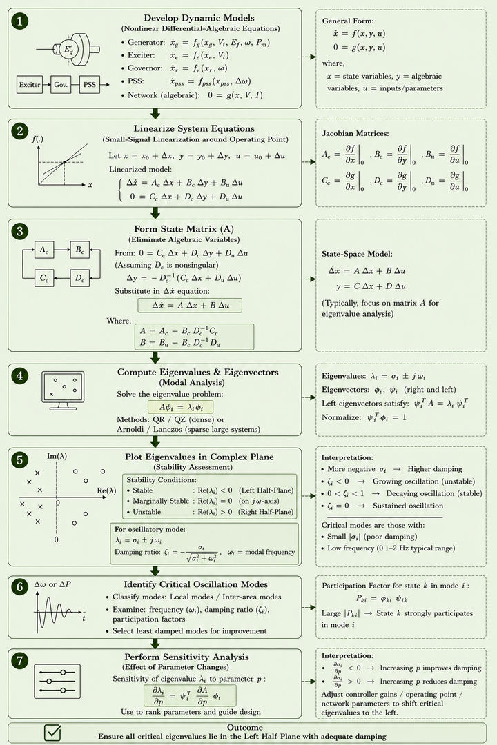
Figure 3: Modal analysis workflow for small signal stability
Impact of Renewable Energy Resources
Declining inertia. Replacing synchronous generators with inverter-based resources lowers system inertia, causing faster frequency changes and making oscillatory modes more sensitive and potentially less damped.
Grid-following inverters. These use PLLs whose behaviour depends on grid strength. In weak grids, interactions between PLL and voltage controls and high source impedance can produce poorly damped oscillations in the 2–20 Hz range.
Grid-forming inverters. These establish voltage and frequency references and can emulate inertia and damping, but they require appropriate energy storage, tuning, and coordination with other resources.
Grid-Following vs Grid-Forming Inverters
Both converter approaches introduce control dynamics that need to be represented explicitly in small signal stability models. Their stability behaviour differs because the control references and dominant loops are different.
| Aspect | Grid-following inverter | Grid-forming inverter |
|---|---|---|
| Control reference | Uses PLL-based synchronization and current-control loops | Sets voltage and frequency references using droop or virtual synchronous control |
| SSS consideration | Weak-grid PLL and voltage-control interactions can introduce poorly damped modes | Can provide inertia-like and damping behaviour, but inappropriate settings can still create oscillatory modes |
| Modelling focus | PLL dynamics, inner current control, outer power/voltage regulation, DC-link and filters | Virtual inertia or droop states, voltage-source emulation, inner voltage/current loops, DC-link and filters |
Sub-Synchronous Control Interaction (SSCI). This is a fast electrical control interaction in converter and series-compensated networks that can cause rapidly growing oscillations and requires detailed converter models for analysis.
Combined stability degradation mechanism. Small signal stability can deteriorate through reduced synchronizing and damping torque, adverse fast converter interactions, weak-grid effects, and the interaction of slower electromechanical dynamics with faster converter controls.
Stability Enhancement Techniques
The following techniques are commonly used to improve small signal stability by increasing damping or controlling the oscillatory behaviour identified through the study.
| Technique | Main purpose | Working | Preferred for | Strengths | Limitations |
|---|---|---|---|---|---|
| Power System Stabilizer (PSS) | Damps local oscillations | Adds supplementary control to excitation system using signals like speed, power, or frequency | Local modes in generator-rich systems | Widely used, effective, mature, low cost. Response time: 0.1–1 s | Hard to tune for multiple modes and changing operating conditions |
| FACTS-based damping controller | Improves damping and power-flow control | Uses SVC, STATCOM, or TCSC to inject control signals and modulate voltage/power flow | Inter-area oscillations and strategic network locations | Flexible placement, good controllability, can use PMU signals. Response time: 10–100 ms | Needs careful coordination and controller design |
| HVDC control | Dampens oscillations through active power modulation | Adjusts power transfer on LCC or VSC-HVDC links to counter oscillations | Inter-area modes across connected regions | Very fast response, strong damping capability. Response time: 5–50 ms | Effective mainly where HVDC exists and requires coordination |
| Wide-area damping controller (WADC) | Coordinates damping over large systems | Uses synchronized PMU measurements for remote, real-time control | Wide-area oscillations in large grids | Better observability, coordinated multi-device action. Response time: 100–500 ms | Communication delay, cybersecurity, and infrastructure dependence |
Where a Small Signal Stability Study Fits in Grid Connection
For renewable projects, small signal stability is one part of the broader power system studies package used to understand grid connection and compliance. Depending on the project scope and applicable network requirements, it may sit alongside load flow, short-circuit, harmonic, and other dynamic studies.
The value of the study is not limited to confirming whether a mode is sufficiently damped. Eigenvalues and participation factors also help identify which equipment or control states are driving the behaviour and where controller tuning or stabilizing measures may be most effective.
SgurrEnergy approaches small signal stability as part of its independent grid and power systems advisory work for renewable projects. The objective is to give developers, IPPs, utilities, lenders, and asset owners a technically grounded view of stability risk and its implications for project decisions.
AI, Machine Learning, and Future Research Trends
Data-driven modal identification. PMU-based methods such as matrix pencil, dynamic model decomposition, and subspace identification can estimate oscillatory modes directly from measurements, while deep learning can improve robustness to noise and missing data.
AI-assisted stability prediction. Machine learning and physics-informed networks can be used to predict stability margins and critical eigenvalues from operating conditions, supporting faster stability assessment.
Reinforcement learning for adaptive control. Reinforcement learning can adapt PSS and FACTS settings online, although practical deployment still faces safety, stability, and regulatory challenges.
Digital twins and edge intelligence. Digital twins combined with edge computing can support real-time stability monitoring, predictive analysis, and decentralized corrective actions.
Research gaps. Key challenges include scalable analysis for converter-dominated grids, a unified treatment of multiple timescales, certified AI controllers, coordination across heterogeneous resources, and probabilistic stability assessment under uncertainty.
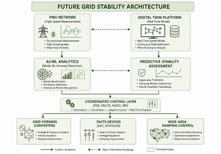
Figure 4: Conceptual architecture for AI-enhanced grid stability management
Conclusion
Small signal stability analysis provides a structured way to understand oscillatory behaviour in both single-machine and multi-machine power systems. By linearizing the system around an operating point and examining eigenvalues, engineers can identify critical or poorly damped modes, determine oscillation frequency and damping, and use eigenvectors and participation factors to understand which states and machines are most involved. These results support controller placement and tuning, help distinguish local and inter-area behaviour, and provide evidence against the applicable stability requirements.
As power systems become more converter-dominated, the importance of this analysis extends beyond classical generator oscillations. Grid-following and grid-forming controls, weak-grid conditions, HVDC and FACTS interactions, and sub-synchronous control interaction can introduce additional modes that need to be understood across relevant operating conditions. For project stakeholders, the practical objective is to identify stability risk early enough to support sound grid-connection, control, and project decisions.
SgurrEnergy positions small signal stability within the wider grid and power systems assessment required for renewable projects. As an independent global renewable energy consultant, SgurrEnergy brings an independent engineering perspective to the interpretation of study outcomes for developers, IPPs, utilities, lenders, and asset owners across the project lifecycle.
For project teams assessing grid connection, dynamic performance, or oscillatory stability, SgurrEnergy’s Grid & Power Systems team can support the study scope and interpretation with an independent engineering perspective.
References
Kundur, P. Power System Stability and Control, McGraw-Hill, 1994.
Anderson, P. M., and Fouad, A. A. Power System Control and Stability, 2nd ed., IEEE Press/Wiley, 2003.
Mondal, D., Chakraborty, A., and Sengupta, A. Power System Small Signal Stability Analysis and Control, 2nd ed., Academic Press, 2020.
Zhang, J., et al. “Modelling and analysis approaches for small-signal stability of converter-dominated networks,” Wiley Interdisciplinary Reviews: Energy and Environment, 2022.
DIgSILENT PowerFactory, 2026 User manual
Authored by
Reena Khanna
Frequently Asked Questions
Small signal stability is the ability of a power system to maintain synchronism following small disturbances. It is assessed around an operating point to determine whether oscillations decay, persist, or grow.
The system is linearized around a selected operating point and represented in state-space form. Eigenvalue analysis is then used to identify oscillatory modes, damping, and frequency, while participation factors show which states are most involved in each mode.
Higher use of inverter-based resources changes system inertia, grid strength, and control interactions. Grid-following and grid-forming converters introduce fast control loops that can interact with the network and create additional oscillatory modes.
Participation factors indicate how strongly individual states contribute to a particular mode. They help identify the machines or control states most involved in a critical oscillation and support controller placement and tuning.
Small signal stability considers small disturbances and uses linearized, eigenvalue-based methods. Transient stability considers large disturbances and requires nonlinear time-domain simulation.
A power system stabilizer provides a supplementary input to a generator excitation system. When correctly tuned, it adds damping to rotor oscillations.
Sub-synchronous control interaction is a fast electrical control interaction that can occur in converter and series-compensated networks. It can produce rapidly growing oscillations and requires detailed converter models for assessment.
The requirement depends on the applicable grid code, system operator, and project-specific grid-connection scope. Where required, the study is used to demonstrate acceptable oscillatory behaviour and to identify poorly damped modes before connection or commissioning.